Mendelian randomisation (MR)
Project status: Complete
Roadmap
- Theory: Document the statistical foundations of Mendelian Randomization (MR), specifically focusing on the Inverse-Variance Weighted (IVW) estimator that uses summary statistics from genome-wide association studies (GWAS).
- Simulation: Set up a simulation framework to generate synthetic data for validating the IVW method.
- Development: Architect and implement a Python package for IVW estimation.
- Automation: Configure a CI/CD pipeline for automated testing and deployment to PyPI.
Theory
Mendelian Randomization is a method that leverages genetic variants as instrumental variables (IV) to infer causal relationships between exposures and outcomes in observational data. The core principle of MR is based on Mendel's laws of inheritance, which suggest that alleles are randomly assorted during gamete formation, thus mimicking the randomization process in randomised controlled trials (RCTs). There are many reviews on MR, e.g., Lawlor et al. (2008), Davey Smith and Hemani (2014), Sanderson et al. (2022), to name a few. The following notes only cover the basics to set the stage for implementation.
Exposures
These are also referred to as modifiable exposures or risk factors. In the context of MR, exposures are the variables that we are interested in studying for their potential causal effect on an outcome. It is essential that the exposure of interest is determined by genetic variants that can be used as IV. For example, if we are interested in studying the causal effect of body mass index (BMI) on cardiovascular disease, BMI would be the exposure.
Outcomes
In MR, outcomes are typically health-related traits or diseases that may be influenced by the exposure. For example, if we are studying the causal effect of BMI on cardiovascular disease, cardiovascular disease would be the outcome.
Instrumental Variables (IV)
In MR, genetic variants are used as IVs (or instruments). They must be associated with the exposure, and must not affect the outcome directly — their influence on the outcome should operate only through their effect on the exposure. Statistical methods using instrumental variables to estimate causal effects were first developed in econometrics in the 1920s, long before the concept of MR was introduced.
Comparison with Randomized Controlled Trials (RCTs)
MR shares some similarities with RCTs in that both methods aim to infer causal relationships between exposures and outcomes. However, unlike RCTs, which involve the random assignment of participants to treatment or control groups, MR relies on the natural random assortment of genetic variants. That is, the chance that an individual inherits a particular genetic variant is random and independent of confounding factors. Thus, if the genetic variant at a locus is associated with the exposure, and if the exposure is causally related to the outcome, then the genetic variant should also be associated with the outcome. As a concrete example, imagine a locus with alleles A and a, where allele A is associated with higher BMI, such that the average BMI of individuals with the AA genotype is higher than those with the Aa genotype, which in turn is higher than those with the aa genotype. If BMI is causally related to cardiovascular disease, then we would expect to see a similar pattern of association between the genotypes and the risk of cardiovascular disease.
A significant advantage of MR over RCTs is that MR can be conducted using existing observational data, which is often more readily available and less expensive than conducting a new RCT. Additionally, MR can provide insights into the long-term effects of exposures, which may not be feasible in RCTs due to time constraints.
Mathematical principles of MR
Let \(X\) be the exposure, \(Y\) be the outcome. The question of interest is whether \(X\) has a causal effect on \(Y\). This can be represented using a directed acyclic graph (DAG) as follows:
Establishing causality from \(X\) to \(Y\) is challenging. For instance, although it is easy to test whether \(X\) and \(Y\) are correlated, correlation does not imply causation. Another common issue is confounding, where a third variable \(U\) influences both \(X\) and \(Y\), leading to a spurious association between \(X\) and \(Y\). An example of this is the relationship between smoking and lung cancer, where socioeconomic status could be a confounder. In this case, individuals with lower socioeconomic status may be more likely to smoke and also have a higher risk of lung cancer due to factors such as limited access to healthcare and increased exposure to environmental pollutants. This may in turn lead to higher rates of lung cancer among smokers, even if we were to assume smoking itself is not the direct cause of lung cancer (despite the fact that it is). This can be represented in a DAG as follows, where a question mark is used to indicate that the causal relationship between \(X\) and \(Y\) is uncertain:
The key idea of MR is to use genetic variants (\(G\)) as IVs. If \(G\) is associated with \(X\) but has no direct effect on \(Y\), then if we observe an association between \(G\) and \(Y\), we can infer that \(X\) has a causal effect on \(Y\). This can be represented in a DAG as follows:
The confounder \(U\) is not a problem in this case because \(G\) is independent of \(U\) (due to the random assortment of alleles during reproduction). This is analogous to the randomization process in RCTs, where assignment to treatment or control groups is independent of confounding factors, and the outcome is only influenced by the treatment assignment.
For simplicity, assume that both \(X\) and \(Y\) are quantitative traits and can be modelled using standard linear models:
where \(\alpha\) and \(\gamma^*\) are intercepts, \(\beta_{GX}\) is the effect of the genetic variant on the exposure, \(\beta_{XY}\) is the causal effect of the exposure on the outcome, and \(\epsilon_X\) and \(\epsilon_Y^*\) are error terms, where \(E(\epsilon_X) = E(\epsilon_Y^*) = 0\). Substituting the equation for \(X\) into the equation for \(Y\), we can derive the following relationship:
Defining \(\gamma = \gamma^* + \beta_{XY} \alpha\), \(\epsilon_Y = \beta_{XY} \epsilon_X + \epsilon_Y^*\), and \(\beta_{GY} = \beta_{XY} \beta_{GX}\), we can rewrite the equation for \(Y\) as:
Thus, if we have estimates \(\widehat{\beta}_{GX}\) and \(\widehat{\beta}_{GY}\), we can estimate the causal effect \(\beta_{XY}\) as
Genome-wide association studies (GWAS) allow for the quantification of associations between a genetic variant and traits \(X\) and \(Y\), yielding the estimates \(\widehat{\beta}_{GX}\) and \(\widehat{\beta}_{GY}\). When data from multiple unlinked genetic variants are available, the above equation suggests that the data points \((\widehat{\beta}_{GX}^{(1)}, \widehat{\beta}_{GY}^{(1)})\), \((\widehat{\beta}_{GX}^{(2)}, \widehat{\beta}_{GY}^{(2)})\), ..., \((\widehat{\beta}_{GX}^{(L)}, \widehat{\beta}_{GY}^{(L)})\) should lie on a line with slope \(\widehat{\beta}_{XY}\), where the superscript denotes the index of the genetic variant. This means that, with GWAS summary statistics widely available, we can combine data from multiple variants from multiple GWASs to obtain a more precise estimate of \(\widehat{\beta}_{XY}\), so long as these different studies are from comparable populations, such that if we were able to test for association between the genetic variants and the traits of interest across all these studies, the causal effect estimates are the same across the studies (bar differences caused by differences in sample sizes). One common method for combining multiple estimates this is the Inverse-Variance Weighted (IVW) estimator, detailed below.
The Inverse-Variance Weighted (IVW) estimator
The causal effect estimates obtained from different genetic variants vary in precision due to differences in sample sizes and allele frequencies. The IVW estimator is a method for combining these estimates that gives more weight to those with higher precision (i.e., lower variance). Let \(\sigma_{GX}^{(i)}\) and \(\sigma_{GY}^{(i)}\) be the standard errors of \(\widehat{\beta}_{GX}^{(i)}\) and \(\widehat{\beta}_{GY}^{(i)}\), respectively. For notational clarity, we will drop the superscript \((i)\) in the following. The variance of the ratio estimator \(\widehat{\beta}_{XY} = \widehat{\beta}_{GY} / \widehat{\beta}_{GX}\) can be approximated using the delta method as follows:
When the estimates \(\widehat{\beta}_{GX}\) and \(\widehat{\beta}_{GY}\) are obtained from independent samples, the covariance term is zero. Further, the estimate \(\widehat{\beta}_{GX}\) is often much more precise than \(\widehat{\beta}_{GY}\) (i.e., \(\sigma_{GX}^2\) is much smaller than \(\sigma_{GY}^2\)). When these two conditions hold, we have
Weighting each estimate \(\widehat{\beta}_{XY}^{(i)}\) by the inverse of its variance, we can obtain the IVW estimator as follows (Burgess et al., 2013):
where \(L\) is the number of genetic variants used as IVs. The variance of the IVW estimator can be estimated as follows:
Let \(z = \widehat{\beta}_{XY}^{(\text{IVW})} / \sqrt{\text{Var}(\widehat{\beta}_{XY}^{(\text{IVW})})}\) be the test statistic for testing the null hypothesis that \(X\) has no causal effect on \(Y\) (i.e., \(\beta_{XY} = 0\)). Under the null hypothesis, \(z^2\) follows a chi-squared distribution with 1 degree of freedom, which can be used to obtain a p-value for the test.
Limitations of the IVW estimator
As is the case for any MR estimators, the validity of the IVW estimator relies on the genetic variants used as IVs satisfying the core assumptions of MR, which are reviewed in detail in, e.g., Sanderson et al. (2022). For the IVW estimator, because it combines estimates from multiple genetic variants, it will be biased even if only one of the genetic variants violates the core assumptions of MR. There are methods for addressing this issue (e.g., Bowden et al., 2016), but they are beyond the scope of this project.
Simulation
In this section, we will set up a simulation framework to generate synthetic data for validating the IVW method. First, consider the exposure \(X\). Without loss of generality, we assume \(\text{Var}(X) = 1\). For simplicity, we assume that \(X\) is influenced by mutations at \(L_X\) independent loci, where each locus has two alleles (0 and 1). Let \(G_X^{(i)}\) be the genotype at the \(i\)-th locus, which can take values of 0, 1, or 2, representing the number of copies of allele 1. We can model \(X\) as follows:
where \(\beta_{GX}^{(i)}\) is the effect of the genotype at the \(i\)-th locus on the exposure, and \(\epsilon_X\) is an error term that follows a normal distribution with mean zero and variance \(\sigma_X^2\). Assuming that the effect sizes and the genotypes are independent, the variance of \(X\) can be expressed as follows:
The heritability of \(X\) is given by
where the second equality follows from the assumption that \(\text{Var}(X) = 1\).
Under the assumption of Hardy-Weinberg equilibrium, the variance of \(G_X^{(i)}\) can be calculated as \(2 p_i (1 - p_i)\), where \(p_i\) is the allele frequency of allele 1 at the \(i\)-th locus. We assume that the mutations are all neutral. Using classical population genetics theory, the allele frequency \(p_i\) can be sampled from a distribution that is proportional to \(1/p_i\) (i.e., the site frequency spectrum). Because GWAS are more appropriate for studying common variants, we restrict our attention to variants with allele frequencies ranging from 0.01 to 0.99. Thus, the expected variance of \(G_X^{(i)}\) can be calculated as follows:
For the effect sizes \(\beta_{GX}^{(i)}\), we can assume that they are drawn from a normal distribution with mean zero and variance \(\sigma_{GX}^2\). Thus, the expected variance of \(X\) can be calculated as follows:
For the outcome \(Y\), we similarly assume \(\text{Var}(Y) = 1\). The variance of \(Y\) can be expressed as follows:
where \(\sigma_Y^2 = \text{Var}(\epsilon_Y)\) is the variance of the normally-distributed error term in the model for \(Y\). Because \(\text{Var}(X) = 1\), the proportion of variance in \(Y\) explained by \(X\) is \(\beta_{XY}^2\).
The inputs for the IVW estimator, \(\widehat{\beta}_{GX}^{(i)}\) and \(\widehat{\beta}_{GY}^{(i)}\), can be simulated directly, without simulating the genotypes. These estimators are based on the simple linear regression model \(y = \beta x + \epsilon\), where \(\epsilon\) is a normally-distributed error term with mean zero and variance \(\sigma^2\). Using the standard large sample approximation, we have \(\widehat{\beta} \sim N\big[\beta, \sigma^2 / (n \text{Var}(x))\big]\), where \(n\) is the sample size (see also notes in my Rust linear regression project). For \(\widehat{\beta}_{GX}^{(i)}\), we use the following assumptions: (1) \(\text{Var}(X) = 1\); (2) \(L_X\) is large and the effect sizes \(\beta_{GX}^{(i)}\) are small; (3) Hardy-Weinberg equilibrium holds. With these assumptions, \(\sigma^2 \approx 1\) and \(\widehat{\beta}_{GX}^{(i)} \sim N\big[\beta_{GX}^{(i)}, (2 n_X p_i (1 - p_i))^{-1}\big]\), where \(n_X\) is the sample size. Similarly, since \(\text{Var}(Y) = 1\) and the individual effects of genetic variants on \(Y\) are small, we have \(\widehat{\beta}_{GY}^{(i)} \sim N\big[\beta_{GY}^{(i)}, (2 n_Y p_i (1 - p_i))^{-1}\big]\), where \(n_Y\) is the sample size and \(\beta_{GY}^{(i)} = \beta_{GX}^{(i)} \beta_{XY}\). For simplicity, the variances of the distributions from which \(\widehat{\beta}_{GX}^{(i)}\) and \(\widehat{\beta}_{GY}^{(i)}\) are sampled are treated as the variances of these estimators.
Simulation procedure
The input parameters are \(L_X\), \(h_X^2\), \(\beta_{XY}\), \(n_X\), \(n_Y\), and \(L_{\text{IV}}\) (the number of IVs). Optionally, the user can also specify a \(p\)-value threshold (denoted as \(p_{\text{threshold}}\)) for selecting IVs.
- Use \(h_X^2\) and \(L_X\) to calculate \(\sigma_{GX}^2\).
- For each of the \(L_{\text{IV}}\) loci,
- Sample the allele frequency \(p_i\) and the effect size \(\beta_{GX}^{(i)}\) from their respective distributions.
- Sample \(\widehat{\beta}_{GX}^{(i)}\) and \(\widehat{\beta}_{GY}^{(i)}\) from their respective distributions.
- Compute \(z_{GX}^{(i)} = \widehat{\beta}_{GX}^{(i)} / \sigma_{GX}^{(i)}\) and \(z_{GY}^{(i)} = \widehat{\beta}_{GY}^{(i)} / \sigma_{GY}^{(i)}\), where \(\sigma_{GX}^{(i)}\) and \(\sigma_{GY}^{(i)}\) are the standard errors of \(\widehat{\beta}_{GX}^{(i)}\) and \(\widehat{\beta}_{GY}^{(i)}\), respectively.
- Compute the \(p\)-values for testing the null hypotheses of no association (i.e., \(\beta_{GX}^{(i)} = 0\) or \(\beta_{GY}^{(i)} = 0\), respectively) by using the fact that \(z_{GX}^{(i)2}\) and \(z_{GY}^{(i)2}\) follow a chi-squared distribution with 1 degree of freedom under the null hypothesis.
- If \(p_{\text{threshold}}\) is specified, reject the simulated data point if the \(p\)-value for testing the null hypothesis of \(\beta_{GX}^{(i)} = 0\) is greater than \(p_{\text{threshold}}\). This mimics the common practice in real data analysis of selecting IVs based on their association with the exposure.
- The output is a TSV file with columns
effect_allele_frequency,true_beta_gx,true_beta_gy,beta_gx,beta_gy,standard_error_beta_gx,standard_error_beta_gy,p_value_beta_gx,p_value_beta_gy.
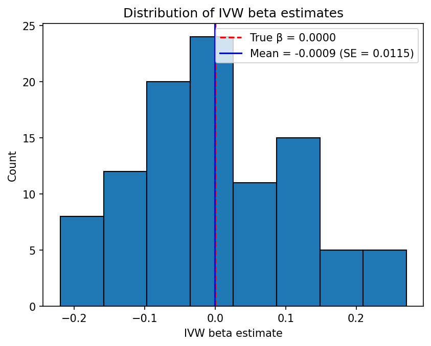
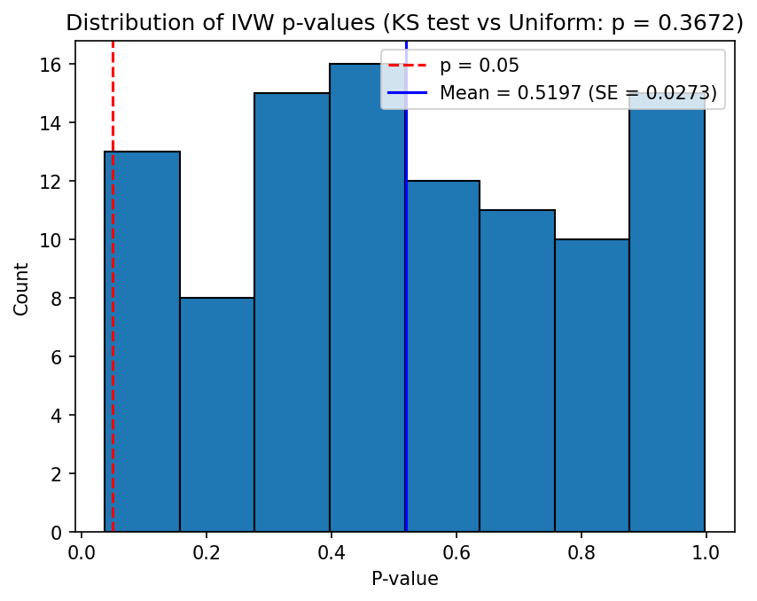
Example 1: Null hypothesis (no causal effect)
This example tests the behaviour of the IVW estimator when the exposure has no causal effect on the outcome (\(\beta_{XY} = 0\)), corresponding to simulations/config_null.json. The simulation parameters are:
- \(h_X^2 = 0.5\), \(L_X = 5000\), giving \(\sigma_{GX}^2 = 0.5 / (0.2133 \times 5000) \approx 4.688 \times 10^{-4}\)
- \(\beta_{XY} = 0\) (0% of the variance in \(Y\) is explained by \(X\))
- \(n_X = 50000\), \(n_Y = 5000\)
- \(L_{\text{IV}} = 100\) loci chosen at random (no \(p\)-value filtering)
Under the null hypothesis, the IVW beta estimates should be centred around zero, and the distribution of p-values should be approximately uniform on \([0, 1]\). The Kolmogorov-Smirnov test can be used to check whether the p-values deviate significantly from uniformity.
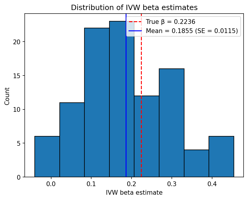
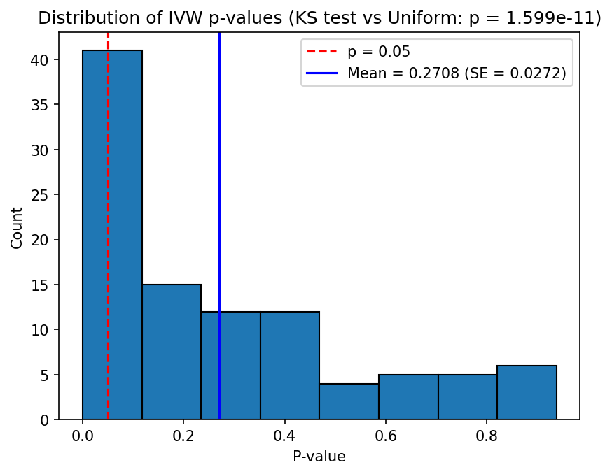
Example 2: Causal effect present
This example tests whether the IVW estimator can recover a true causal effect, corresponding to simulations/config.json. The simulation parameters are:
- \(h_X^2 = 0.5\), \(L_X = 5000\), giving \(\sigma_{GX}^2 = 0.5 / (0.2133 \times 5000) \approx 4.688 \times 10^{-4}\)
- 5% of the variance in \(Y\) is explained by \(X\), so \(\beta_{XY} = \sqrt{0.05} \approx 0.2236\)
- \(n_X = 50000\), \(n_Y = 5000\)
- \(L_{\text{IV}} = 100\) loci chosen at random (no \(p\)-value filtering)
The IVW beta estimates should be centred around the true \(\beta_{XY} \approx 0.2236\), and the p-values should be concentrated near zero (rejecting the null hypothesis of no causal effect). In contrast to Example 1, the Kolmogorov-Smirnov test should reject uniformity of the p-values.
Installation
Usage
As a CLI tool
Assume that an environment with the package installed has been activated.
Simulate GWAS summary statistics
simulate \
    --exposure-heritability 0.5 \
    --exposure-num-causal-variants 5000 \
    --num-instrumental-variables 100 \
    --exposure-sample-size 50000 \
    --outcome-sample-size 5000 \
    --percent-outcome-variance-explained-by-exposure 5 \
    --seed 42 \
    --output-tsv simulated.tsv
Estimate causal effect using IVW
As an importable library
from numpy.random import default_rng

from mendelian_randomisation.estimate import ivw_estimate
from mendelian_randomisation.simulate import run_simulation

rng = default_rng(42)
sim_result = run_simulation(
    exposure_heritability=0.5,
    exposure_num_causal_variants=5000,
    num_instrumental_variables=100,
    exposure_sample_size=50000,
    outcome_sample_size=5000,
    percent_outcome_variance_explained_by_exposure=5,
    rng=rng,
)

result = ivw_estimate(
    sim_result["beta_gx"],
    sim_result["beta_gy"],
    sim_result["standard_error_beta_gy"],
)
print(f"IVW beta: {result.beta:.4f} (SE: {result.standard_error:.4f})")
Note that simulate and estimate are functions decorated with @click.command(), which turns them into click.core.Command objects. To call the underlying function directly, use the .callback attribute.
References
Bowden, J., Davey Smith, G., Haycock, P.C. and Burgess, S., 2016. Consistent estimation in Mendelian randomization with some invalid instruments using a weighted median estimator. Genetic epidemiology, 40(4), pp.304-314.
Burgess, S., Butterworth, A. and Thompson, S.G., 2013. Mendelian randomization analysis with multiple genetic variants using summarized data. Genetic epidemiology, 37(7), pp.658-665.
Davey Smith, G. and Hemani, G., 2014. Mendelian randomization: genetic anchors for causal inference in epidemiological studies. Human molecular genetics, 23(R1), pp.R89-R98.
Lawlor, D.A., Harbord, R.M., Sterne, J.A., Timpson, N. and Davey Smith, G., 2008. Mendelian randomization: using genes as instruments for making causal inferences in epidemiology. Statistics in medicine, 27(8), pp.1133-1163.
Sanderson, E., Glymour, M.M., Holmes, M.V., Kang, H., Morrison, J., Munafò, M.R., Palmer, T., Schooling, C.M., Wallace, C., Zhao, Q. and Davey Smith, G., 2022. Mendelian randomization. Nature reviews Methods primers, 2(1), p.6.